Introduction
For a real life working example, we have this dataset graciously provided to us by the National Institute of Standards and Technology (http://www.nist.gov/) for one of their test bed parts. We will be trying to solve the first example from the introduction, which was a real problem faced by the NIST researchers. As we walk through each step of the exploratory process, you will understand how you can use similar techniques to solve similar issues that you might have with your Machine Tools.
Problem Statement
Accurately estimate the productive time of a part, from the data of a part that was manufactured with interruptions. Productive time is defined as the time taken by the machine to complete the part excluding interruptions and inefficiencies.
Reading Data into R
First let us define the data files that we are going to be working with. Two sets of example data from the MTConnect Agent samples and the result of the MTConnect probe are provided along with the package. We will be using the one provided by NIST for this analysis. Note that the package can read in a compressed file as if it were a normal file as well for the samples.
Taking a quick look at the data files
Before we read in the data into the MTC Device Class, it might help us a bit in understanding a bit about the data items that we have.
Devices XML Data
get_device_info_from_xml
The
MTConnectDevices XML document has information about the logical components of one or more devices. This file can obtained using the
probe request from an MTConnect Agent.
We can check out the devices for which the info is present in the devices XML using the
get_device_info_from_xml function. From the device info, we can select the name of the device that we want to analyse further
get_xpaths_from_xml
The
get_xpath_from_xml function can read in the xpath info for a single device into a easily read data.frame format.
The data.frame contains the id and name of each data item and the xpath along with the type, category and subType of the data_item. It is easy to find out what are the data items of a particular type using this function. For example, we are going to find out the conditions data items which we will be using in the next step.
Getting Sample data by parsing
MTConnectStreams data
MTConnectStreams data from an MTConnect Agent can be collected using a
ruby script to generate a delimited log of device data (referred to in this document as
log data) which is then used by the
mtconnectR Package.
Creating MTC Device Class
create_mtc_device_from_dmtcd function can read in both the Delimited MTConnect data (DMTCD) and the xml data for a device and combine it into a single MTCDevice Class with the data organized separately for each data item.
Exploring different data items
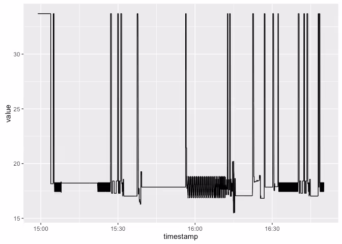
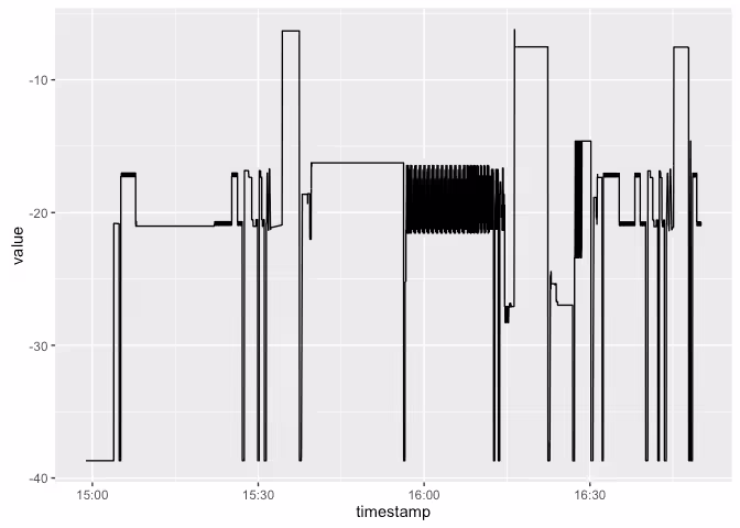
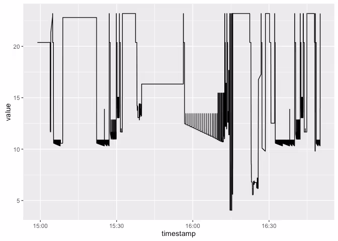
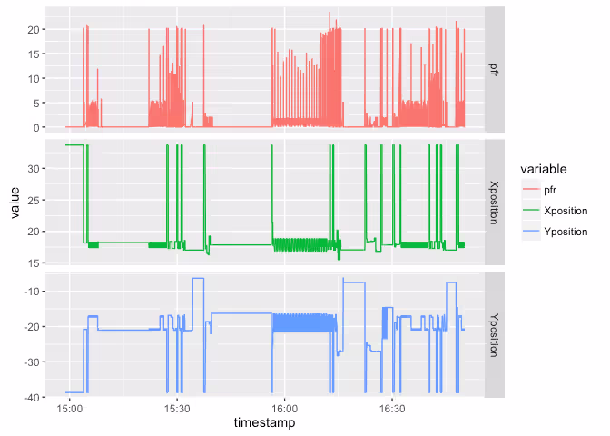
It looks like we have the position data items that we might need for this analysis in the log data. Let's see the variation in position. We can plot all the data items in one plot using ggplot2.
Plotting the data
Merging different data items for simultaneous analysis
It looks like the machine is going back and forth quite some distance quite often, across all the axes. We also don't know how this traversal varies across different axis. However, we can get a much better idea of the motion if we could plot one axis against the other. For that we have to merge the different data items. Since the different data items have different timestamp values as the key, it is not as straightforward as doing a join of one data item against the other. For this purpose, the
mtconnect packge has a merge method defined for the MTCDevice Class
Oops. Looks like we have also merged in the angular position. Let's try a more directed merge. Also, the names of the data items have the full xpaths attached to them. While this might be useful in other circumstances to get the hierarchical position of the data, we can dispense with it now using the
extract_param_from_xpath function. Let's view the data after that
Much better. Now let's plot the data items in one shot.
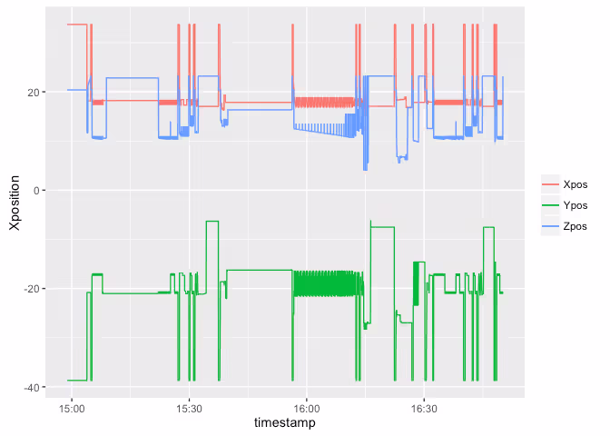
It does look the sudden traverals are simultaenous across the axes. Plotting one axes against the other leads to the same conclusion. It also gives us an idea of the different representations of the part

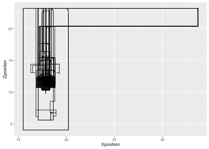
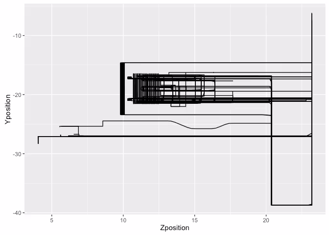
So the machine tool is going to the origin every so often.
Deriving new process parameters
It might help our analysis to also calculate a few process parameters that the machine tool is not providing directly. Here we are going to calculate the actual Path Feedrate of the machine as it executes the process using the position data.
Derived Path Feedrate
Path Feedrate can be calculated as the rate of change of the position values. Here, we must use the 3-dimensional distance value and not just one of the position vectors.
PFR = Total Distance / Total Time = Sqrt(Sum of Squares of distane along individual axis) / time taken for motion
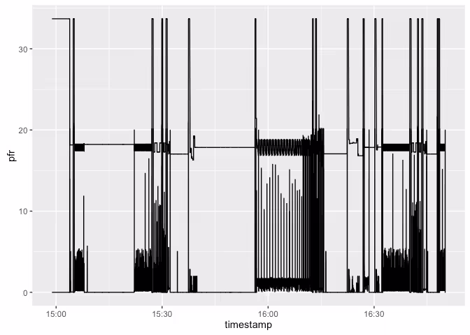
Let's add this derived data back into the MTCDevice Class.
Identifying Inefficiencies
Idle times
Our first task is to identify the periods when the machine was idle. For this we can use a few approaches.
- Find out the times when the execution status was not active OR
- Find out the times when the machine was not feeding (PFR~0) OR
- Find the periods when the feed override was zero
We will be trying out all the approaches and choosing union of the three as the period when machine is idle.
Machine tool at origin
We need to identify the time spent by the machine at origin. Let's look at the X - Y graph again
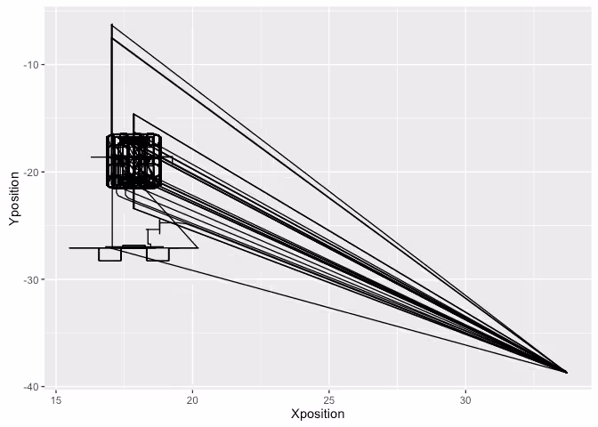
It is clear that the periods when the machine was origin are roughly X > 30, Y < -30. Adding this into the mix
Calculating Summary Statistics
Now we have all the data at our disposal to calculate the time statistics. First we need to convert the time series into interval format to get the duratins. We can use
convert_ts_to_interval function to do the same.
Now we can aggregate across the different states to find the total amount of time in each state.